互联网+

选自3dbabove

参与：乾树、刘晓坤

本文使用通俗的语言和形象的图示，介绍了随机梯度下降算法和它的三种经典变体，并提供了完整的实现代码。

GitHub 链接：https://github.com/ManuelGonzalezRivero/3dbabove

代价函数的多种优化方法

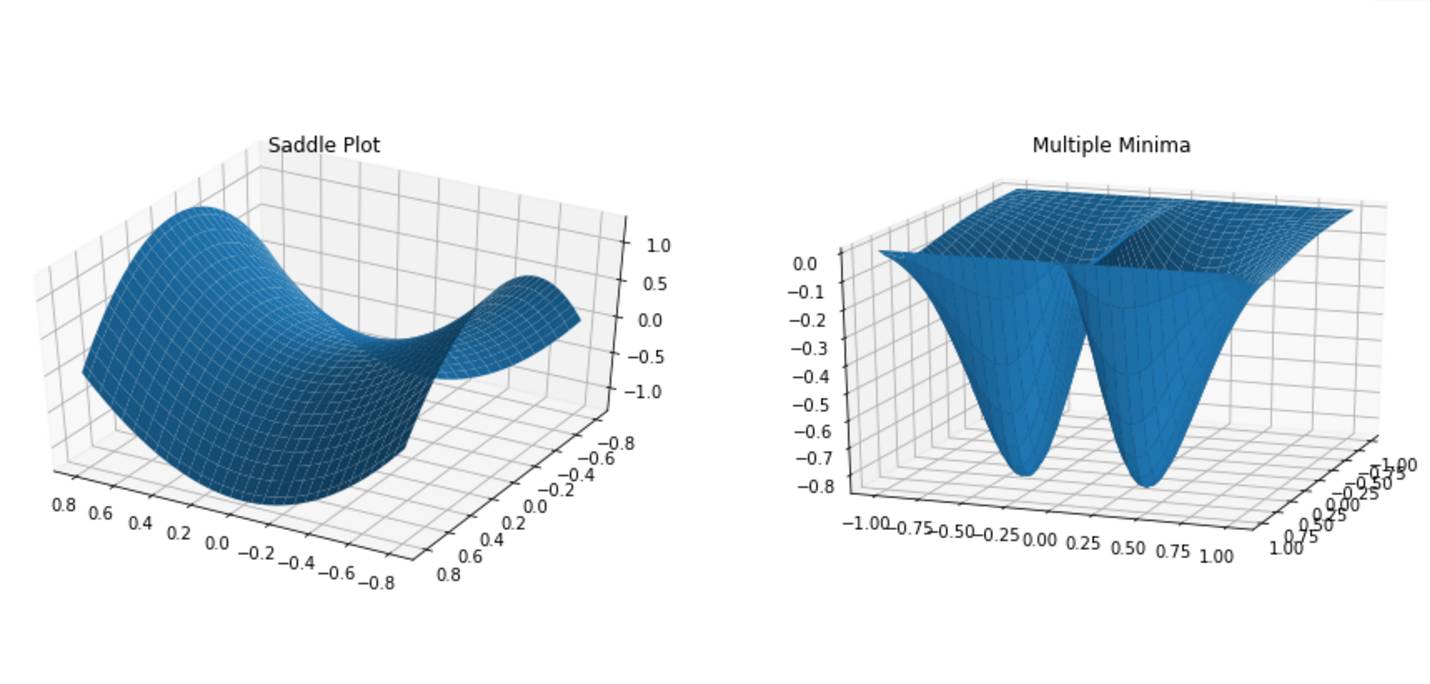
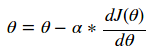
目标函数是衡量预测值和实际值的相似程度的指标。通常，我们希望得到使代价尽可能小的参数集，而这意味着你的算法性能不错。函数的最小可能代价被称为最小值。有时一个代价函数可以有多个局部极小值。幸运的是，在参数空间的维数非常高的情况下，阻碍目标函数充分优化的局部最小值并不经常出现，因为这意味着对象函数相对于每个参数在训练过程的早期都是凹的。但这并非常态，通常我们得到的是许多鞍点，而不是真正的最小值。

找到生成最小值的一组参数的算法被称为优化算法。我们发现随着算法复杂度的增加，则算法倾向于更高效地逼近最小值。我们将在这篇文章中讨论以下算法：

• 随机梯度下降法

• 动量算法

• RMSProp

• Adam 算法

随机梯度下降法

我的「Logistic 回归深入浅出」的文章里介绍了一个随机梯度下降如何运作的例子。如果你查阅随机梯度下降法的资料（SGD），通常会遇到如下的等式：

资料上会说，θ是你试图找到最小化 J 的参数，这里的 J 称为目标函数。最后，我们将学习率记为α。通常要反复应用上述等式，直到达到你所需的代价值。

这是什么意思？想一想，假如你坐在一座山顶上的雪橇上，望着另一座山丘。如果你滑下山丘，你会自然地往下移动，直到你最终停在山脚。如果第一座小山足够陡峭，你可能会开始滑上另一座山的一侧。从这个比喻中你可以想到：

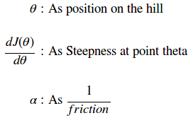
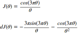
学习率越高意味着摩擦力越小，因此雪橇会像在冰上一样沿着山坡下滑。低的学习率意味着摩擦力高，所以雪橇会像在地毯上一样，难以滑下。我们如何用上面的方程来模拟这种效果？

随机梯度下降法：

1. 初始化参数（θ，学习率）

2. 计算每个θ处的梯度

3. 更新参数

4. 重复步骤 2 和 3，直到代价值稳定

让我们用一个简单的例子来看看它是如何运作的！

在这里我们看到一个目标函数和它的导数（梯度）：

我们可以用下面的代码生成函数和梯度值/30 的图：

1. importnumpy asnp

3. defminimaFunction(theta):

4. returnnp.cos(3*np.pi*theta)/theta

6. defminimaFunctionDerivative(theta):

7. const1 =3*np.pi

8. const2 =const1*theta

9. return-(const1*np.sin(const2)/theta)-np.cos(const2)/theta**2

11. theta =np.arange(.1,2.1,.01)

12. Jtheta=minimaFunction(theta)

13. dJtheta =minimaFunctionDerivative(theta)

15. plt.plot(theta,Jtheta,label =r'$J(theta)$')

16. plt.plot(theta,dJtheta/30,label =r'$dJ(theta)/30$')

17. plt.legend()

18. axes =plt.gca()

19. #axes.set_ylim([-10,10])

21. plt.ylabel(r'$J(theta),dJ(theta)/30$')

22. plt.xlabel(r'$theta$')

23. plt.title(r'$J(theta),dJ(theta)/30 $ vs $theta$')

24. plt.show()

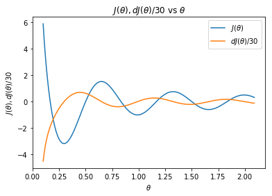
上图中有两个细节值得注意。首先，注意这个代价函数有几个极小值（大约在 0.25、1.0 和 1.7 附近取得）。其次，注意在最小值处的导数在零附近的曲线走向。这个点就是我们所需要的新参。

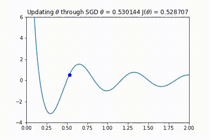
我们可以在下面的代码中看到上面四个步骤的实现。它还会生成一个视频，显示每个步骤的θ和梯度的值。

1. importnumpy asnp

2. importmatplotlib.pyplot asplt

3. importmatplotlib.animation asanimation

5. defoptimize(iterations,oF,dOF,params,learningRate):

6. """

7. computes the optimal value of params for a given objective function and its derivative

8. Arguments:

9. - iteratoins - the number of iterations required to optimize the objective function

10. - oF - the objective function

11. - dOF - the derivative function of the objective function

12. - params - the parameters of the function to optimize

13. - learningRate - the learning rate

14. Return:

15. - oParams - the list of optimized parameters at each step of iteration

16. """

17. oParams =[params]

18. #The iteration loop

19. fori inrange(iterations):

20. # Compute the derivative of the parameters

21. dParams =dOF(params)

22. # Compute the update

23. params =params-learningRate*dParams

25. # app end the new parameters

26. oParams.append(params)

28. returnnp.array(oParams)

30. defminimaFunction(theta):

31. returnnp.cos(3*np.pi*theta)/theta

33. defminimaFunctionDerivative(theta):

34. const1 =3*np.pi

35. const2 =const1*theta

36. return-(const1*np.sin(const2)/theta)-np.cos(const2)/theta**2

38. theta =.6

39. iterations=45

40. learningRate =.0007

41. optimizedParameters =optimize(iterations,

42. minimaFunction,

43. minimaFunctionDerivative,

44. theta,

45. learningRate)

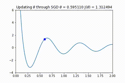
这似乎运作得很好！您应该注意到，如果θ的初始值较大，则优化算法将在某一个局部极小处结束。然而，如上所述，在极高维度空间中这种可能性并不大，因为它要求所有参数同时满足凹函数。

你可能会想，「如果我们的学习率太大，会发生什么？」。如果步长过大，则算法可能永远不会找到如下的动画所示的最佳值。监控代价函数并确保它单调递减，这一点很重要。如果没有单调递减，可能需要降低学习率。

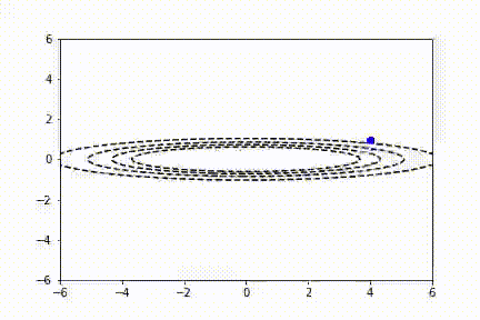
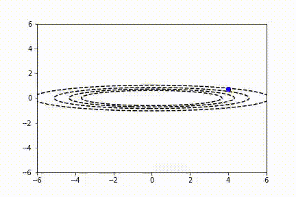
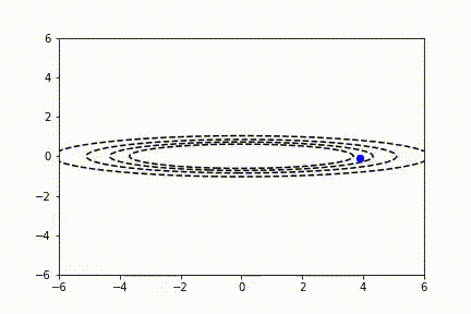
SGD 也适用于多变量参数空间的情况。我们可以将二维函数绘制成等高线图。在这里你可以看到 SGD 对一个不对称的碗形函数同样有效。

1. importnumpy asnp

2. importmatplotlib.mlab asmlab

3. importmatplotlib.pyplot asplt

4. importscipy.stats

5. importmatplotlib.animation asanimation

7. defminimaFunction(params):

8. #Bivariate Normal function

9. X,Y =params

11. sigma11,sigma12,mu11,mu12 =(3.0,.5,0.0,0.0)

13. Z1 =mlab.bivariate_normal(X,Y,sigma11,sigma12,mu11,mu12)

15. Z =Z1

17. return-40*Z

19. defminimaFunctionDerivative(params):

20. # Derivative of the bivariate normal function

21. X,Y =params

23. sigma11,sigma12,mu11,mu12 =(3.0,.5,0.0,0.0)

25. dZ1X =-scipy.stats.norm.pdf(X,mu11,sigma11)*(mu11 -X)/sigma11**2

26. dZ1Y =-scipy.stats.norm.pdf(Y,mu12,sigma12)*(mu12 -Y)/sigma12**2

28. return(dZ1X,dZ1Y)

30. defoptimize(iterations,oF,dOF,params,learningRate,beta):

31. """

32. computes the optimal value of params for a given objective function and its derivative

33. Arguments:

34. - iteratoins - the number of iterations required to optimize the objective function

35. - oF - the objective function

36. - dOF - the derivative function of the objective function

37. - params - the parameters of the function to optimize

38. - learningRate - the learning rate

39. - beta - The weighted moving average parameter

40. Return:

41. - oParams - the list of optimized parameters at each step of iteration

42. """

43. oParams =[params]

44. vdw =(0.0,0.0)

45. #The iteration loop

46. fori inrange(iterations):

47. # Compute the derivative of the parameters

48. dParams =dOF(params)

50. #SGD in this line Goes through each parameter and applies parameter = parameter -learningrate*dParameter

51. params =tuple([par-learningRate*dPar fordPar,par inzip(dParams,params)])

53. # append the new parameters

54. oParams.append(params)

56. returnoParams

58. iterations=100

59. learningRate =1

60. beta =.9

61. x,y =4.0,1.0

62. params =(x,y)

63. optimizedParameters =optimize(iterations,

64. minimaFunction,

65. minimaFunctionDerivative,

66. params,

67. learningRate,

68. beta)

动量 SGD

注意，传统 SGD 没有解决所有问题！通常，用户想要使用非常大的学习速率来快速学习感兴趣的参数。不幸的是，当代价函数波动较大时，这可能导致不稳定。你可以看到，在前面的视频中，由于缺乏水平方向上的最小值，y 参数方向的抖动形式。动量算法试图使用过去的梯度预测学习率来解决这个问题。通常，使用动量的 SGD 通过以下公式更新参数：

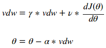
γ 和 ν 值允许用户对 dJ(θ) 的前一个值和当前值进行加权来确定新的θ值。人们通常选择γ和ν的值来创建指数加权移动平均值，如下所示：

β参数的最佳选择是 0.9。选择一个等于 1-1/t 的β值可以让用户更愿意考虑νdw 的最新 t 值。这种简单的改变可以使优化过程产生显著的结果！我们现在可以使用更大的学习率，并在尽可能短的时间内收敛！

1. importnumpy asnp

2. importmatplotlib.mlab asmlab

3. importmatplotlib.pyplot asplt

4. importscipy.stats

5. importmatplotlib.animation asanimation

7. defminimaFunction(params):

8. #Bivariate Normal function

9. X,Y =params

11. sigma11,sigma12,mu11,mu12 =(3.0,.5,0.0,0.0)

13. Z1 =mlab.bivariate_normal(X,Y,sigma11,sigma12,mu11,mu12)

15. Z =Z1

17. return-40*Z

19. defminimaFunctionDerivative(params):

20. # Derivative of the bivariate normal function

21. X,Y =params

23. sigma11,sigma12,mu11,mu12 =(3.0,.5,0.0,0.0)

25. dZ1X =-scipy.stats.norm.pdf(X,mu11,sigma11)*(mu11 -X)/sigma11**2

26. dZ1Y =-scipy.stats.norm.pdf(Y,mu12,sigma12)*(mu12 -Y)/sigma12**2

28. return(dZ1X,dZ1Y)

30. defoptimize(iterations,oF,dOF,params,learningRate,beta):

31. """

32. computes the optimal value of params for a given objective function and its derivative

33. Arguments:

34. - iteratoins - the number of iterations required to optimize the objective function

35. - oF - the objective function

36. - dOF - the derivative function of the objective function

37. - params - the parameters of the function to optimize

38. - learningRate - the learning rate

39. - beta - The weighted moving average parameter for momentum

40. Return:

41. - oParams - the list of optimized parameters at each step of iteration

42. """

43. oParams =[params]

44. vdw =(0.0,0.0)

45. #The iteration loop

46. fori inrange(iterations):

47. # Compute the derivative of the parameters

48. dParams =dOF(params)

50. # Compute the momentum of each gradient vdw = vdw*beta+(1.0+beta)*dPar

51. vdw =tuple([vDW*beta+(1.0-beta)*dPar fordPar,vDW inzip(dParams,vdw)])

53. #SGD in this line Goes through each parameter and applies parameter = parameter -learningrate*dParameter

54. params =tuple([par-learningRate*dPar fordPar,par inzip(vdw,params)])

56. # append the new parameters

57. oParams.append(params)

59. returnoParams

61. iterations=100

62. learningRate =5.3

63. beta =.9

64. x,y =4.0,1.0

65. params =(x,y)

66. optimizedParameters =optimize(iterations,

67. minimaFunction,

68. minimaFunctionDerivative,

69. params,

70. learningRate,

71. beta)

RMSProp

像工程中的其它事物一样，我们一直在努力做得更好。RMS prop 试图通过观察关于每个参数的函数梯度的相对大小，来改善动量函数。因此，我们可以取每个梯度平方的加权指数移动平均值，并按比例归一化梯度下降函数。具有较大梯度的参数的 sdw 值将变得比具有较小梯度的参数大得多，从而使代价函数平滑下降到最小值。可以在下面的等式中看到：

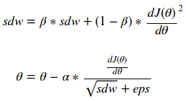
请注意，这里的 epsilon 是为数值稳定性而添加的，可以取 10e-7。这是为什么昵？

1. importnumpy asnp

2. importmatplotlib.mlab asmlab

3. importmatplotlib.pyplot asplt

4. importscipy.stats

5. importmatplotlib.animation asanimation

7. defminimaFunction(params):

8. #Bivariate Normal function

9. X,Y =params

11. sigma11,sigma12,mu11,mu12 =(3.0,.5,0.0,0.0)

13. Z1 =mlab.bivariate_normal(X,Y,sigma11,sigma12,mu11,mu12)

15. Z =Z1

17. return-40*Z

19. defminimaFunctionDerivative(params):

20. # Derivative of the bivariate normal function

21. X,Y =params

23. sigma11,sigma12,mu11,mu12 =(3.0,.5,0.0,0.0)

25. dZ1X =-scipy.stats.norm.pdf(X,mu11,sigma11)*(mu11 -X)/sigma11**2

26. dZ1Y =-scipy.stats.norm.pdf(Y,mu12,sigma12)*(mu12 -Y)/sigma12**2

28. return(dZ1X,dZ1Y)

30. defoptimize(iterations,oF,dOF,params,learningRate,beta):

31. """

32. computes the optimal value of params for a given objective function and its derivative

33. Arguments:

34. - iteratoins - the number of iterations required to optimize the objective function

35. - oF - the objective function

36. - dOF - the derivative function of the objective function

37. - params - the parameters of the function to optimize

38. - learningRate - the learning rate

39. - beta - The weighted moving average parameter for RMSProp

40. Return:

41. - oParams - the list of optimized parameters at each step of iteration

42. """

43. oParams =[params]

44. sdw =(0.0,0.0)

45. eps =10**(-7)

46. #The iteration loop

47. fori inrange(iterations):

48. # Compute the derivative of the parameters

49. dParams =dOF(params)

51. # Compute the momentum of each gradient sdw = sdw*beta+(1.0+beta)*dPar^2

52. sdw =tuple([sDW*beta+(1.0-beta)*dPar**2fordPar,sDW inzip(dParams,sdw)])

54. #SGD in this line Goes through each parameter and applies parameter = parameter -learningrate*dParameter

55. params =tuple([par-learningRate*dPar/((sDW**.5)+eps)forsDW,par,dPar inzip(sdw,params,dParams)])

57. # append the new parameters

58. oParams.append(params)

60. returnoParams

62. iterations=10

63. learningRate =.3

64. beta =.9

65. x,y =5.0,1.0

66. params =(x,y)

67. optimizedParameters =optimize(iterations,

68. minimaFunction,

69. minimaFunctionDerivative,

70. params,

71. learningRate,

72. beta)

Adam 算法

Adam 算法将动量和 RMSProp 的概念结合成一种算法，以获得两全其美的效果。公式如下：

1. importnumpy asnp

2. importmatplotlib.mlab asmlab

3. importmatplotlib.pyplot asplt

4. importscipy.stats

5. importmatplotlib.animation asanimation

7. defminimaFunction(params):

8. #Bivariate Normal function

9. X,Y =params

11. sigma11,sigma12,mu11,mu12 =(3.0,.5,0.0,0.0)

13. Z1 =mlab.bivariate_normal(X,Y,sigma11,sigma12,mu11,mu12)

15. Z =Z1

17. return-40*Z

19. defminimaFunctionDerivative(params):

20. # Derivative of the bivariate normal function

21. X,Y =params

23. sigma11,sigma12,mu11,mu12 =(3.0,.5,0.0,0.0)

25. dZ1X =-scipy.stats.norm.pdf(X,mu11,sigma11)*(mu11 -X)/sigma11**2

26. dZ1Y =-scipy.stats.norm.pdf(Y,mu12,sigma12)*(mu12 -Y)/sigma12**2

28. return(dZ1X,dZ1Y)

30. defoptimize(iterations,oF,dOF,params,learningRate,beta1,beta2):

31. """

32. computes the optimal value of params for a given objective function and its derivative

33. Arguments:

34. - iteratoins - the number of iterations required to optimize the objective function

35. - oF - the objective function

36. - dOF - the derivative function of the objective function

37. - params - the parameters of the function to optimize

38. - learningRate - the learning rate

39. - beta1 - The weighted moving average parameter for momentum component of ADAM

40. - beta2 - The weighted moving average parameter for RMSProp component of ADAM

41. Return:

42. - oParams - the list of optimized parameters at each step of iteration

43. """

44. oParams =[params]

45. vdw =(0.0,0.0)

46. sdw =(0.0,0.0)

47. vdwCorr =(0.0,0.0)

48. sdwCorr =(0.0,0.0)

50. eps =10**(-7)

51. #The iteration loop

52. fori inrange(iterations):

53. # Compute the derivative of the parameters

54. dParams =dOF(params)

56. # Compute the momentum of each gradient vdw = vdw*beta+(1.0+beta)*dPar

57. vdw =tuple([vDW*beta1+(1.0-beta1)*dPar fordPar,vDW inzip(dParams,vdw)])

59. # Compute the rms of each gradient sdw = sdw*beta+(1.0+beta)*dPar^2

60. sdw =tuple([sDW*beta2+(1.0-beta2)*dPar**2.0fordPar,sDW inzip(dParams,sdw)])

61. # Compute the weight boosting for sdw and vdw

62. vdwCorr =tuple([vDW/(1.0-beta1**(i+1.0))forvDW invdw])

63. sdwCorr =tuple([sDW/(1.0-beta2**(i+1.0))forsDW insdw])

65. #SGD in this line Goes through each parameter and applies parameter = parameter -learningrate*dParameter

66. params =tuple([par-learningRate*vdwCORR/((sdwCORR**.5)+eps)forsdwCORR,vdwCORR,par inzip(vdwCorr,sdwCorr,params)])

68. # append the new parameters

69. oParams.append(params)

71. returnoParams

73. iterations=100

74. learningRate =.1

75. beta1 =.9

76. beta2 =.999

77. x,y =5.0,1.0

78. params =(x,y)

79. optimizedParameters =optimize(iterations,

80. minimaFunction,

81. minimaFunctionDerivative,

82. params,

83. learningRate,

84. beta1,

85. beta2)</div>

Adam 算法可能是目前深度学习中使用最广泛的优化算法，适用于多种应用。Adam 计算了一个 νdw^corr 的值，用于加快指数加权移动平均值的变化。它将通过增加它们的值来对它们进行标准化，与当前的迭代次数成反比。使用 Adam 时有一些很好的初始值可供尝试。它最好以 0.9 的 β_1 和 0.999 的 β_2 开头。

总结

优化目标函数的算法有相当多的选择。在上述示例中，我们发现各种方法的收敛速度越来越快：

– SGD: 100 次迭代

– SGD+Momentum: 50 次迭代

– RMSProp: 10 次迭代

– ADAM: 5 次迭代

原文链接：https://3dbabove.com/2017/11/14/optimizationalgorithms/

本文为机器之心编译，转载请联系本公众号获得授权。返回搜狐，查看更多

责任编辑：